customised stochastic simulations

Customised stochastic simulations

The ThermoGIS methodology calculate_doublet_performance_stochastic assumes that we know the net-to-gross, porosity and depth of the aquifer and simulates doublets over a range of values for transmissivity (calculated from permeability and thickness). There are two main reasons for selecting this statistical framework:

1. It is fast as we only sample over one parameter (and for the ThermoGIS website we have to run a lot of simulations)
2. Transmissivity affects doublet performance significantly while often having a relatively high uncertainty

However, if conducting a local study you may well want to explore a model space across other reservoir properties, or develop your own statistical framework. Luckily, it is easy (and insightful) to use pythermogis to generate samples and make your own stochastic framework. Here is a simple example where you define probability distributions on your input parameters and then run simulations across random combinations of those input parameters before deriving statistics from those simulations:

from pythermogis import calculate_doublet_performance, calculate_pos, plot_exceedance
import xarray as xr
from matplotlib import pyplot as plt
from pathlib import Path
from os import path
import numpy as np


# output directory to write output to
output_data_path = Path(path.dirname(__file__), "resources") / "test_output" / "exceedance_example"
output_data_path.mkdir(parents=True, exist_ok=True)

# generate simulation samples across desired reservoir properties
Nsamples = 1000
thickness_samples = np.random.uniform(low=150, high=300, size=Nsamples)
porosity_samples = np.random.uniform(low=0.5, high=0.8, size=Nsamples)
ntg_samples = np.random.uniform(low=0.25, high=0.5, size=Nsamples)
depth_samples = np.random.normal(loc=2000, scale=100, size=Nsamples)
permeability_samples = np.random.normal(loc=400, scale=100, size=Nsamples)
reservoir_properties = xr.Dataset(
    {
        "thickness": (["sample"], thickness_samples),
        "porosity": (["sample"], porosity_samples),
        "ntg": (["sample"], ntg_samples),
        "depth": (["sample"], depth_samples),
        "permeability": (["sample"], permeability_samples),
    },
    coords={"sample": np.arange(Nsamples)}
)

# For every sample, run a doublet simulation store the output values
simulations = calculate_doublet_performance(reservoir_properties, print_execution_duration=True)

# post process the samples to calculate the percentiles of each variable
percentiles = np.arange(1,99)
results = simulations.quantile(q=percentiles/100, dim="sample")
results = results.assign_coords(quantile=("quantile", percentiles)) # Overwrite the 'quantile' coordinate with integer percentiles
results = results.rename({"quantile": "p_value"}) # Rename dimension to 'p_value' to match nomenclature in the rest of pythermogis
results["pos"] = calculate_pos(results)

# plotting
fig, axes = plt.subplots(3,2, figsize=(10,15))
plt.suptitle("Reservoir Property Distributions")
reservoir_properties.thickness.plot.hist(ax=axes[0,0])
reservoir_properties.porosity.plot.hist(ax=axes[0,1])
reservoir_properties.ntg.plot.hist(ax=axes[1,0])
reservoir_properties.depth.plot.hist(ax=axes[1,1])
reservoir_properties.permeability.plot.hist(ax=axes[2,0])
axes[2,1].set_visible(False)
plt.savefig(output_data_path / "reservoir_distributions.png")

fig, axes = plt.subplots(2,2, figsize=(10,10))
plt.suptitle(f"Simulation results\nNo. of Samples: {Nsamples}")
simulations.plot.scatter(x="permeability", y="transmissivity", ax=axes[0,0])
simulations.plot.scatter(x="permeability", y="utc", ax=axes[0,1])
simulations.plot.scatter(x="permeability", y="power", ax=axes[1,0])
simulations.plot.scatter(x="permeability", y="npv", ax=axes[1,1])
plt.savefig(output_data_path / "simulation_results.png")

fig, axes = plt.subplots(2,2, figsize=(10,10))
plt.suptitle(f"Exceedance probability curves\nNo. of Samples: {Nsamples}")
plot_exceedance(results["permeability"], ax=axes[0,0])
plot_exceedance(results["utc"], ax=axes[0,1])
plot_exceedance(results["power"], ax=axes[1,0])
plot_exceedance(results["npv"], ax=axes[1,1])
axes[1, 1].axhline(results["pos"], ls="--", c="tab:orange", label=f"POS: {results["pos"]:.1f}%")   # add the probability of success
axes[1, 1].axvline(0, ls="--", c="tab:orange")  # add the probability of success
axes[1, 1].legend()
plt.savefig(output_data_path / "exceedance_probabilities.png")

Firstly, we define how many simulations we want to run (1000 simulations takes approximately 10 seconds on an average laptop). Then we define the range of values we want our simulations to test, here thickness, porosity and net-to-gross are defined as uniform distributions while permeability and depth are normal distributions. We generate samples for each reservoir property and construct a Dataset with the dimension samples:

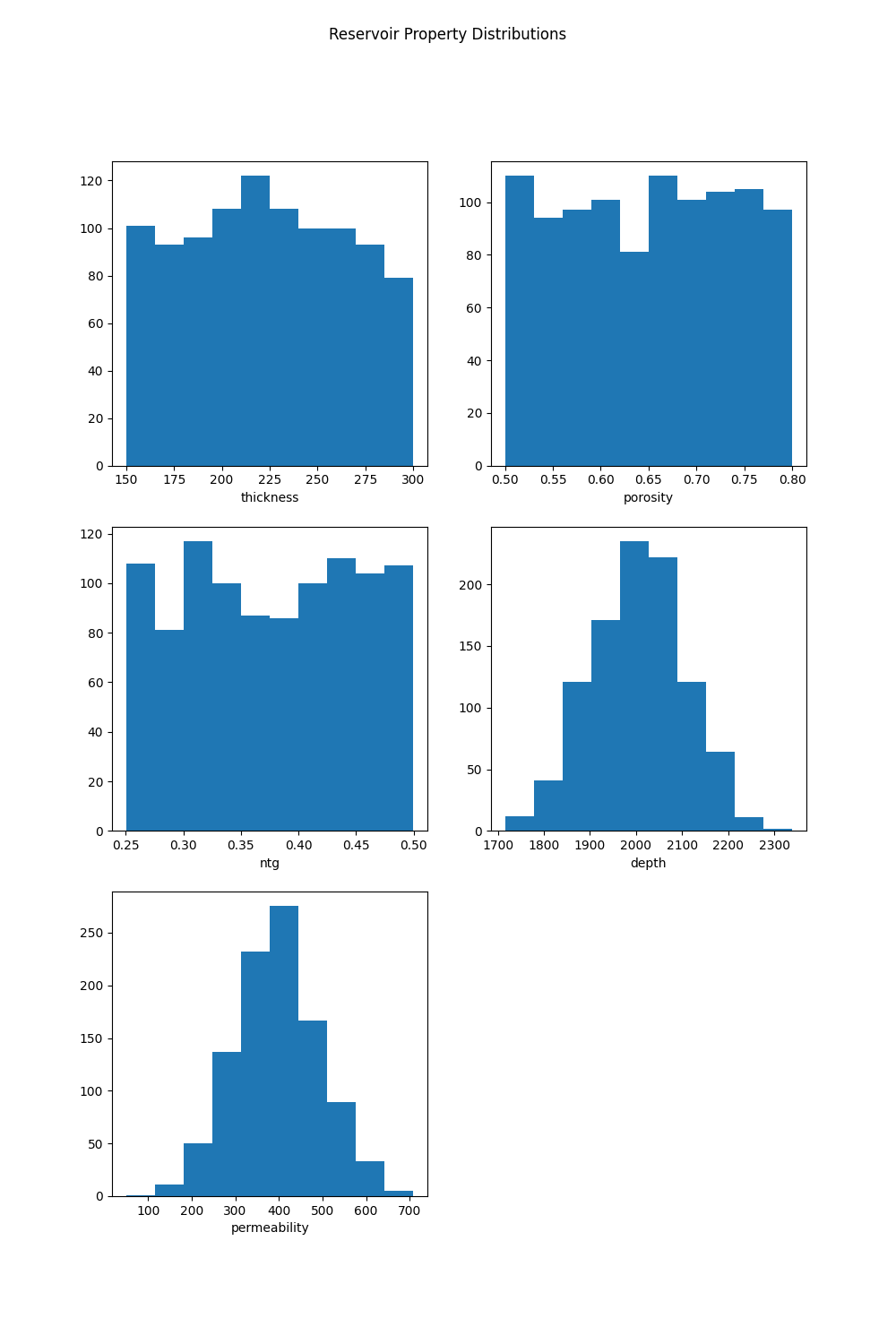
Figure: The sampled distributions for each reservoir property

Then 1000 simulations are run and outputted to the simulations Dataset:

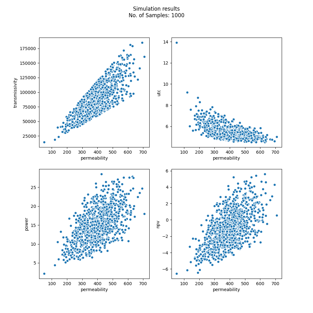
Figure: Distribution of simulation results across a few parameters of interest

And then from these samples percentiles are calculated across each output parameter, from which exceedance probability graphs can be made:

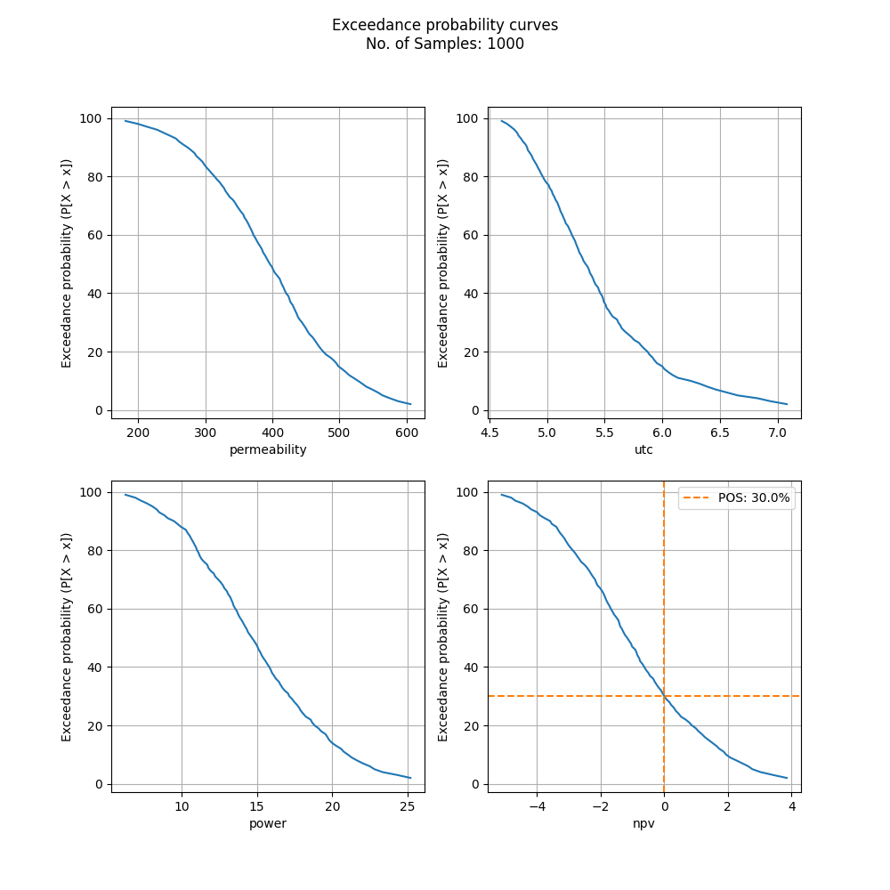
Figure: Exceedance probabilities; for example this shows that their is a 30% chance that net-present-value is greater than 0