Depth Optimization
This is an example of how to use the calculate_doublet_performance function from
the pythermogis package to run the simulation for a range of transmissivity values across depth in an aquifer.
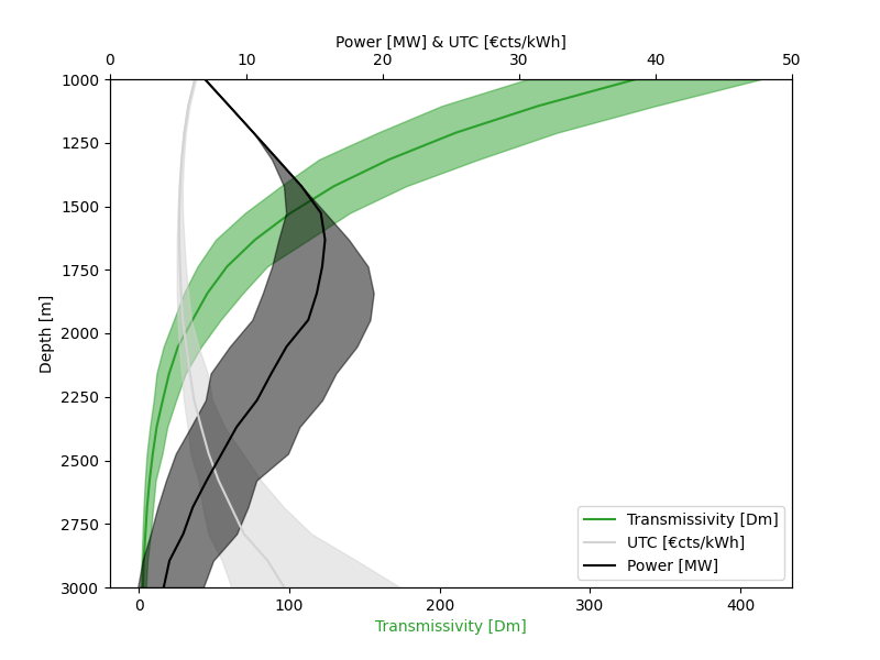
The final result then allows for optimal assesment of where to place a Doublet system in depth for a single location.
This relies on the following information:
- an estimate of the vertical extent of the aquifer and the uncertainty of that estimate
- an estimate of the porosity-depth relationship of the aquifer and the uncertainty of the relationship
- an estimate of the porosity-permeability relationship of the aquifer and the uncertainty of the relationship
Combining these variables allows a stochastic model to be made combining the uncertainties in these parameters which highlights the correlations between transmissivty, depth, unit technical cost and power output:
The code used to make this plot is as follows (and is the same as test_example9 in test_doc_examples.py in the test suite of the repo.)
from pathlib import Path

import numpy as np
import xarray as xr
from matplotlib import pyplot as plt

from pythermogis import calculate_doublet_performance

# output directory to write output to
output_data_path = Path(__file__).parent.parent / "resources" / "test_output" / "example9"
output_data_path.mkdir(parents=True, exist_ok=True)

# define the poro-depth and the poro-perm relationships:
# porosity = (poro_0-poro_base) * exp(-poro_k * depth) + poro_base, with depth in km
# values below correspond to the Sirte Basin
poro_0 = 45
poro_k = 0.4
poro_b = 4.0
poro_std = 1  # 0.01% uncertainty, if this goes larger it blows up massively...

# ln(permeability) =
# porperm: [-0.0092, 0.76, -6.7]
perm_a = -0.0092
perm_b = 0.76
perm_c = -6.7

# number of depths and number of samples per depth
n_samples = 500
n_depths = 20


depth_min = 1e3
depth_max = 3e3
depths = np.linspace(depth_min, depth_max, n_depths)
thickness = 100
ntg = 1.0

porosity = (poro_0-poro_b) * np.exp(-poro_k * (depths * 1e-3)) + poro_b

# expand porosity to have n_samples per depth, with uncertainty in porosity
porosity = np.random.normal(porosity[:, None], poro_std, size=(n_depths, n_samples))
porosity = np.clip(porosity, 0.0, 100.0)

permeability = np.exp(perm_a * porosity**2 + perm_b * porosity +  perm_c)
# clip to minimum transmissivity of 1Dm
permeability = np.clip(permeability, 1000/thickness, 1e10)

reservoir_properties = xr.Dataset(
    {
        "thickness": thickness,
        "porosity": (["depth", "samples"], porosity / 100),
        "ntg": ntg,
        "permeability": (["depth", "samples"], permeability),
    },
    coords={
        "samples": np.arange(n_samples),
        "depth": depths,
    },
)


# For every sample, run a doublet simulation
simulations = calculate_doublet_performance(
    reservoir_properties,
    chunk_size=100,
)


simulations_stoch = simulations.quantile([0.1,0.5,0.9], dim="samples")


# make a plot showing there is a sweet spot between Doublet power, Cost of energy
# and Transmissivity
fig, ax = plt.subplots(figsize=(8, 6))
ax2 = ax.twiny()

p10 = simulations_stoch.sel(quantile=0.9)
p50 = simulations_stoch.sel(quantile=0.5)
p90 = simulations_stoch.sel(quantile=0.1)


# UTC
ax2.fill_betweenx(p50.depth, p10.utc, p90.utc, color="lightgrey", alpha=0.5)
ax2.plot(p50.utc, p50.depth, label="UTC [€cts/kWh]", color="lightgrey")
ax2.set_xlim(0,50)

# power
ax2.fill_betweenx(p50.depth, p10.power, p90.power, color="black", alpha=0.5)
ax2.plot(p50.power, p50.power.depth, label="Power [MW]", color="black")

# transmissivity
ax.fill_betweenx(
    p50.depth,
    p10.transmissivity_with_ntg,
    p90.transmissivity_with_ntg,
    color="tab:green",
    alpha=0.5,
)
ax.plot(
    p50.transmissivity_with_ntg,
    p50.transmissivity_with_ntg.depth,
    label="Transmissivity [Dm]",
    color="tab:green",
)

ax.set_ylabel("Depth [m]")
ax2.set_xlabel("Power [MW] & UTC [€cts/kWh]")
ax.set_xlabel("Transmissivity [Dm]", color="tab:green")
ax.set_ylim([depths[-1], depths[0]])

# Collect handles and labels from both axes
handles1, labels1 = ax.get_legend_handles_labels()
handles2, labels2 = ax2.get_legend_handles_labels()
handles = handles1 + handles2
labels = labels1 + labels2
ax.legend(handles, labels)

plt.savefig(output_data_path / "depth_optimization.png")