Depth Optimization
This is an example of how to use the ThermoGISDoublet class from
the pythermogis package to run the simulation for a range of transmissivity values across depth in an aquifer.
The final result then allows for optimal assesment of where to place a Doublet system in depth for a single location.
This relies on the following information:
- an estimate of the vertical extent of the aquifer and the uncertainty of that estimate
- an estimate of the porosity-depth relationship of the aquifer and the uncertainty of the relationship
- an estimate of the porosity-permeability relationship of the aquifer and the uncertainty of the relationship
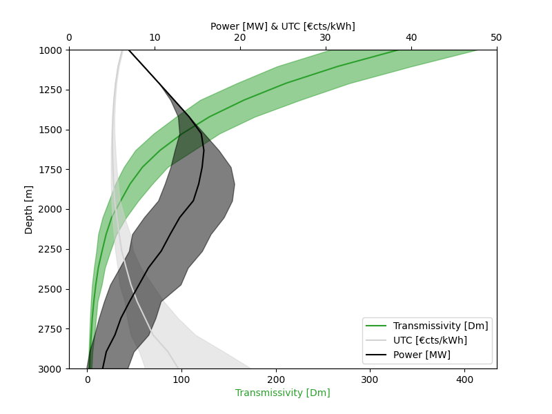
Combining these variables allows a stochastic model to be made combining the uncertainties in these parameters which highlights the correlations between transmissivty, depth, unit technical cost and power output:
The code used to make this plot is as follows (and is the same as test_example9 in test_doc_examples.py in the test suite of the repo.)
from pathlib import Path

import numpy as np
import xarray as xr
from matplotlib import pyplot as plt

from pythermogis.aquifer import Aquifer
from pythermogis.doublet import ThermoGISDoublet

# output directory to write output to
output_data_path = Path("test_output") / "example9"
output_data_path.mkdir(parents=True, exist_ok=True)

# define the poro-depth and the poro-perm relationships:
# porosity = (poro_0-poro_base) * exp(-poro_k * depth) + poro_base, with depth in km
# values below correspond to the Sirte Basin
poro_0 = 45
poro_k = 0.4
poro_b = 4.0
poro_std = 1  # 0.01% uncertainty, if this goes larger it blows up massively...

# ln(permeability) =
# porperm: [-0.0092, 0.76, -6.7]
perm_a = -0.0092
perm_b = 0.76
perm_c = -6.7

# number of depths and number of samples per depth
n_samples = 500
n_depths = 20


depth_min = 1e3
depth_max = 3e3
depths = np.linspace(depth_min, depth_max, n_depths)
thickness = 100
ntg = 1.0

porosity = (poro_0 - poro_b) * np.exp(-poro_k * (depths * 1e-3)) + poro_b

# expand porosity to have n_samples per depth, with uncertainty in porosity
porosity = np.random.normal(porosity[:, None], poro_std, size=(n_depths, n_samples))
porosity = np.clip(porosity, 0.0, 100.0)

permeability = np.exp(perm_a * porosity**2 + perm_b * porosity + perm_c)
# clip to minimum transmissivity of 1Dm
permeability = np.clip(permeability, 1000 / thickness, 1e10)

porosity_da = xr.DataArray(
    porosity / 100,
    dims=["depth", "samples"],
    coords={"depth": depths, "samples": np.arange(n_samples)},
)
permeability_da = xr.DataArray(
    permeability,
    dims=["depth", "samples"],
    coords={"depth": depths, "samples": np.arange(n_samples)},
)
depth_da = xr.DataArray(depths, dims=["depth"], coords={"depth": depths})

aquifer = Aquifer(
    thickness=thickness,
    porosity=porosity_da,
    ntg=ntg,
    depth=depth_da,
    permeability=permeability_da,
)


# For every sample, run a doublet simulation
simulations = ThermoGISDoublet(aquifer=aquifer).simulate(chunk_size=100).to_dataset()


simulations_stoch = simulations.quantile([0.1, 0.5, 0.9], dim="samples")


# make a plot showing there is a sweet spot between Doublet power, Cost of energy
# and Transmissivity
fig, ax = plt.subplots(figsize=(8, 6))
ax2 = ax.twiny()

p10 = simulations_stoch.sel(quantile=0.9)
p50 = simulations_stoch.sel(quantile=0.5)
p90 = simulations_stoch.sel(quantile=0.1)


# UTC
ax2.fill_betweenx(p50.depth, p10.utc, p90.utc, color="lightgrey", alpha=0.5)
ax2.plot(p50.utc, p50.depth, label="UTC [€cts/kWh]", color="lightgrey")
ax2.set_xlim(0,50)

# power
ax2.fill_betweenx(p50.depth, p10.power, p90.power, color="black", alpha=0.5)
ax2.plot(p50.power, p50.power.depth, label="Power [MW]", color="black")

# transmissivity
ax.fill_betweenx(
    p50.depth,
    p10.transmissivity_with_ntg,
    p90.transmissivity_with_ntg,
    color="tab:green",
    alpha=0.5,
)
ax.plot(
    p50.transmissivity_with_ntg,
    p50.transmissivity_with_ntg.depth,
    label="Transmissivity [Dm]",
    color="tab:green",
)

ax.set_ylabel("Depth [m]")
ax2.set_xlabel("Power [MW] & UTC [€cts/kWh]")
ax.set_xlabel("Transmissivity [Dm]", color="tab:green")
ax.set_ylim([depths[-1], depths[0]])

# Collect handles and labels from both axes
handles1, labels1 = ax.get_legend_handles_labels()
handles2, labels2 = ax2.get_legend_handles_labels()
handles = handles1 + handles2
labels = labels1 + labels2
ax.legend(handles, labels)

plt.savefig(output_data_path / "depth_optimization.png")