Portfolio run and analysis

Portfolio run and analysis of doublet simulations

This is simple example of how to use the ThermoGISDoublet class from the pythermogis package to run the simulation for a set of maps and p-values.

This example demonstrates the following steps:

1. Reading input grids for:

   • Mean thickness
   • Thickness standard deviation
   • Net-to-gross ratio
   • Porosity
   • Mean permeability
   • Log(permeability) standard deviation

2. define a portfolio of locations on the grid to run the simulation for

3. Running doublet simulations and calculating economic indicators (e.g., power production, CAPEX, NPV) across all non-NaN cells in the input grids for a range of p-values (10% to 90% in 10% increments).

4. Exporting results to file.

5. Plotting result maps for selected p-values (10%, 50%, and 90%) for:

   • Power output
   • Capital expenditure (CAPEX)
   • Net Present Value (NPV)

6. Plotting expectation curves for NPV(POS),KH,power and COP expectation curves at portfolio locations.

Example input data for this workflow is available in the /resources/example_data directory of the repository.

This example corresponds to test case test_example6 in test_doc_examples.py in the tests directory of the repository.

from pathlib import Path

import numpy as np
import xarray as xr
from matplotlib import pyplot as plt
from pygridsio import read_grid

from pythermogis.aquifer import StochasticAquifer
from pythermogis.doublet import ThermoGISDoublet
from pythermogis.postprocess import calculate_pos

input_data_path = Path("test_input") / "example_data"
output_data_path = Path("test_output") / "example7"
output_data_path.mkdir(parents=True, exist_ok=True)

# read in reservoir property maps
thickness_mean = read_grid(input_data_path / "ROSL_ROSLU__thick.zmap")
thickness_sd = read_grid(input_data_path / "ROSL_ROSLU__thick_sd.zmap")
ntg = read_grid(input_data_path / "ROSL_ROSLU__ntg.zmap")
porosity = 0.01 * read_grid(input_data_path / "ROSL_ROSLU__poro.zmap")
depth = read_grid(input_data_path / "ROSL_ROSLU__top.zmap")
ln_permeability_mean = np.log(read_grid(input_data_path / "ROSL_ROSLU__perm.zmap"))
ln_permeability_sd = read_grid(input_data_path / "ROSL_ROSLU__ln_perm_sd.zmap")

aquifer = StochasticAquifer(
    thickness_mean=thickness_mean,
    thickness_sd=thickness_sd,
    ntg=ntg,
    porosity=porosity,
    depth=depth,
    ln_permeability_mean=ln_permeability_mean,
    ln_permeability_sd=ln_permeability_sd,
)

# Select locations of interest from the reservoir properties and simulate
# doublet performance
portfolio_coords = [
    (125e3, 525e3),
    (100e3, 525e3),
    (110e3, 525e3),
    (125e3, 515e3),
    (125e3, 520e3),
]

# Collect selected locations, create a new Dataset with the coordinate 'location'
aquifer_ds = aquifer.to_dataset()

locations = []
for i, (x, y) in enumerate(portfolio_coords):
    point = aquifer_ds.sel(x=x, y=y, method="nearest")
    point = point.expand_dims(location=[i])
    locations.append(point)
portfolio_reservoir_properties = xr.concat(locations, dim="location")

portfolio_aquifer = StochasticAquifer(**portfolio_reservoir_properties.data_vars)

results_portfolio = (
    ThermoGISDoublet(aquifer=portfolio_aquifer)
    .simulate(p_values=[10, 20, 30, 40, 50, 60, 70, 80, 90])
    .to_dataset()
)

# post process: clip the npv and calculate the probability of success
AEC = -3.5
results_portfolio['npv'] = results_portfolio.npv.clip(min=AEC)
results_portfolio["pos"] = calculate_pos(results_portfolio)

# plot results
fig, axes = plt.subplots(ncols=2, nrows=2, figsize=(10, 10))
colors = plt.cm.tab10.colors
for i_loc, loc in enumerate(portfolio_coords):
    # select single portfolio location to plot
    results_loc = results_portfolio.isel(location=i_loc)
    pos = results_loc.pos.data
    x, y = loc

    # plot npv versus p-value and a map showing the location of interest
    ax = axes[0, 0]
    results_loc.npv.plot(y="p_value", ax=ax, color=colors[i_loc])
    ax.set_title("Aquifer: ROSL_ROSLU\n  POS ")
    ax.axhline(
        pos, label=f"POS: {pos:.1f}% [ {x:.0f}m, {y:.0f}m]", ls="--", c=colors[i_loc]
    )
    ax.axvline(0.0, ls="--", c=colors[i_loc])
    ax.legend()
    ax.set_xlabel("net-present-value [Million €]")
    ax.set_ylabel("p-value [%]")

    ax = axes[0, 1]
    kh = results_loc.transmissivity_with_ntg
    kh.plot(y="p_value", ax=ax, color=colors[i_loc])
    ax.set_title("Aquifer: ROSL_ROSLU\n kH")
    temp = results_loc.temperature.sel()
    inj_temp = results_loc.inj_temp.sel(p_value=50)
    prd_temp = results_loc.prd_temp.sel(p_value=50)
    ax.axhline(
        50.0,
        label=f"POS: {pos:.1f}%  TEMP res: {temp:.1f} inj: "
        f"{inj_temp:.1f} prd: {prd_temp:.1f} ",
        ls="--",
        c=colors[i_loc],
    )
    ax.axvline(kh.sel(p_value=50), ls="--", c=colors[i_loc])
    ax.legend()
    ax.set_xlabel("kH [Dm]")
    ax.set_ylabel("p-value [%]")

    ax = axes[1, 0]
    results_loc.power.plot(y="p_value", ax=ax, color=colors[i_loc])
    ax.set_title("Aquifer: ROSL_ROSLU\n Power")
    ax.axhline(
        pos, label=f"POS: {pos:.1f}% [ {x:.0f}m, {y:.0f}m]", ls="--", c=colors[i_loc]
    )
    valp50 = results_loc.power.sel(p_value=50)
    ax.axvline(valp50, ls="--", c=colors[i_loc])
    ax.legend()
    ax.set_xlabel("power [MW]")
    ax.set_ylabel("p-value [%]")

    ax = axes[1, 1]
    results_loc.cop.plot(y="p_value", ax=ax, color=colors[i_loc])
    ax.set_title("Aquifer: ROSL_ROSLU\n COP")
    ax.axhline(
        pos, label=f"POS: {pos:.1f}% [ {x:.0f}m, {y:.0f}m]", ls="--", c=colors[i_loc]
    )
    valp50 = results_loc.cop.sel(p_value=50)
    ax.axvline(valp50, ls="--", c=colors[i_loc])
    ax.legend()
    ax.set_xlabel("COP [-]")
    ax.set_ylabel("p-value [%]")

plt.tight_layout()  # ensure there is enough spacing
plt.savefig(output_data_path / "npv.png")

The figure generated by the above code will look like this:

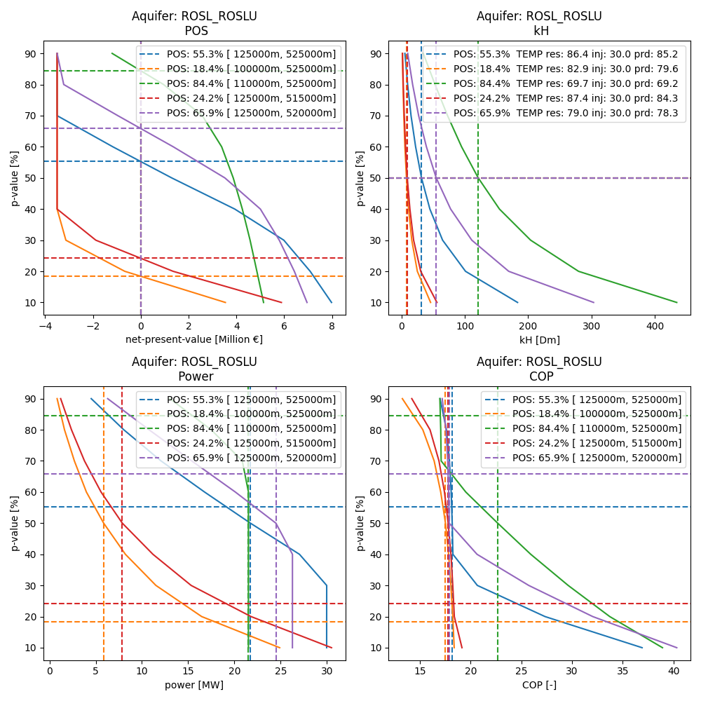Figure: probability of success based on NPV at a single location